Excel's New Dynamic Array Feature

Excel’s new dynamic array feature is one of the best enhancements Microsoft has added to Excel in years. With dynamic arrays, we now have the capability of creating more powerful formulas than ever before. That is, dynamic arrays allow us to break free from the traditional “one-cell, one-formula” paradigm. Instead, we can now have a single formula that places results into many cells. Further, Microsoft has added several new useful functions that return results into these dynamic arrays.

CLICK HERE to learn more about the need for technology focused learning

A Brief History of Array Formulas

As an Excel feature, array formulas are not new. Prior to dynamic arrays, Excel offered traditional array formulas. In that environment, we could create a formula – typically one with several functions nested in it – and then use a CTRL+SHIFT+ENTER (CSE) keyboard sequence to enter the formula into a cell. While these types of formulas were useful – and remain so today – their complexity is overwhelming for most Excel users. Additionally, Excel offers a few functions – SUMPRODUCT, for example – that operates much like a CSE array formula yet does not require the CSE keyboard sequence. Dynamic arrays do not eliminate legacy arrays. Instead, this new feature just means that we have another powerful tool to work with in Excel.

Understanding the Concept of a Dynamic Array

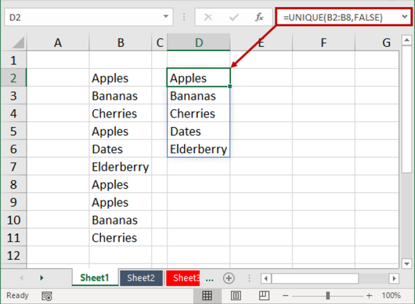
In a preceding paragraph, I mentioned the “one-cell, one-formula” paradigm. Before dynamic arrays, we had to enter formulas into every cell where we wanted calculation results to display. Dynamic arrays change that by allowing us to create a single formula and the results of that single formula will appear in as many cells as necessary, given the volume of data under consideration. To illustrate, consider the example provided in Figure 1. In this example, the formula shown in the formula bar was entered only into cell D2. However, the formula dynamically copied itself to create a listing of all the unique values in the range.

The fundamental example presented above illustrates the concept of a “dynamic array.” More specifically, it provides evidence that dynamic arrays can populate multiple “results” cells even though the formula itself is entered into only a single cell. Importantly, if the source range in the example (B2:B8) had been first converted to a table, then as the volume of data in the table changed, so too would the volume of results in the dynamic array.

New Functions to Capitalize on Dynamic Arrays

To make the concept of dynamic arrays even more useful, Microsoft has released six new functions that capitalize on this model. We list each of these six functions below and have added emphasis to the FILTER and SORT functions, because they are likely to be used most often.

FILTER

As implied by its name, the FILTER function is capable of filtering data in a table or a range via a formula. The syntax is relatively simple, as shown below.

=FILTER(array (table or range), include (a Boolean array for which items to include))

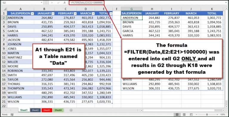
An optional third argument – [if_empty] – specifies the value to display if the filter returns nothing. Figure 2 below displays an example of how you can use the FILTER function to filter data, without disturbing the original array.

RANDARRAY

The RANDARRAY function returns an array of random numbers. The syntax for RANDARRAY follows.

=RANDARRAY([rows],[columns],[min],[max],[whole_number]), where

rows is an optional argument for the number of rows to be returned,
columns is an optional argument for the number of columns to be returned,
min is an optional argument for the smallest number to be returned,
max is an optional argument for the largest number to be returned, and
whole_number is an optional argument for Excel to return TRUE for a whole number and FALSE for a decimal number.

RANDARRAY would be the ideal function to return a row(s) and column(s) of random numbers and serves as a useful alternative to the RAND and RANDBETWEEN functions.

SEQUENCE

You can use the SEQUENCE function to generate a list of sequential numbers displayed in an array. The syntax of the SEQUENCE function is relatively simple, as shown below.

=SEQUENCE(rows, [columns], [start], [step]), where

rows is a required entry for the number of rows in the new array,
columns is an optional argument for the number of columns in the new array,
start, is an optional argument for the first number in the sequence, and
step, is an optional argument for the amount to increment each number in the array.

SORT

You can use SORT to sort a table or range of data based on the values in a specific column. Following is the syntax for the SORT function.

=SORT(array (table or range), Sort_index (column), Sort_order (1 for ascending, -1 for descending))

An optional fourth argument – [by col] exists to allows you to choose the sort direction. By default, the sort direction is by row. If you need to sort by column, you can change that to TRUE.

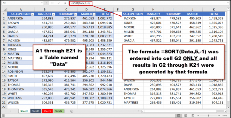
Thus, the formula =SORT(Data,5,-1) sorts the table named Data, based on the values in the fifth column and the sort would be in descending order, as shown in Figure 3.

SORTBY

Excel’s new SORTBY function sorts a range or an array based on the values in a corresponding range or array. The syntax for SORTBY is provided below.

=SORTBY(array, by_array1, [sort_order1], [by_array2, sort_order2],…), where

array is a required argument for the array or range to sort,
by_array1..2..3..etc. is the range or array to sort on,
sort_order1..2..3..etc. is the order to use for sorting, where 1 is ascending (default) and -1 is descending.

UNIQUE

The UNIQUE function identifies and returns a list of all unique values in a list or range. The syntax for the UNIQUE follows.

=UNIQUE(array,[by_col],[exactly_once]), where

array is a required argument from which to return the unique rows or columns,
by_col is an optional argument indicating how to compare. An entry of TRUE will compare columns against each other and return the unique columns and an entry of FALSE (or omitted) will compare rows against each other and return the unique rows, and
exactly_once is an optional, logical argument that will return rows or columns that occur exactly once in the range or array. TRUE will return all distinct rows or columns that occur exactly once and FALSE will return all distinct rows or columns from the range or array.

Unfortunately, Not All Excel Users Will Get This Functionality

Microsoft has started gradually rolling-out dynamic array functionality to Office 365 subscribers on version 1912 of Excel or newer. If you are an Office 365 subscriber, the exact date you will receive an update that contains this feature depends upon your update channel. It is expected that most Office 365 subscribers will receive access to dynamic array functionality in 2020. Presently, there do not appear to be any plans for users of Excel on an existing perpetual license – such as Excel 2019 or 2016 – to receive access to dynamic arrays.

Summary

Dynamic arrays and related dynamic array functions are among the most powerful features ever added to Excel. With their strength and capability to handle large volumes of data easily, they will no doubt prove to be one of the best additions to Excel in years. If you are an Office 365 subscriber, you should be on the lookout for dynamic arrays, because you will likely receive access to them soon. Unfortunately, if you use a perpetual license of Excel, it is unlikely you will gain access to this feature in your current version of Excel.

Excel’s New Dynamic Array Feature