Can You Build Formula-Based PivotTables? Now You Can With PIVOTBY!

For years, I’ve said that PivotTables are Excel’s best feature. Their near-limitless number of ways to summarize without writing formulas allows us to create reports summarizing vast data volumes. However, in some cases, the structure associated with PivotTables limited users. For instance, arranging a PivotTable report into a particular format can be problematic, as can generating calculations in the PivotTable outside of the eleven provided summarization options. Fortunately, Excel’s new PIVOTBY function addresses these issues and allows you the flexibility to build your reports precisely the way you want!
What Is PIVOTBY?
PIVOTBY is a relatively new function in Excel that allows you to create formula-based PivotTable-like reports. PIVOTBY is now available to most Microsoft 365 subscribers to provide reporting options unavailable in traditional PivotTables. Specifically, the function allows you to create reports that aggregate and summarize data based on your specified groupings. Further, because reports based on the function are formula-driven, by default, they will update any time the underlying data changes; of course, this trait means that you no longer need to refresh your PivotTables manually.
Perhaps the most significant feature associated with is that the feature can use virtually any and all of Excel’s functions to perform necessary calculations. Thus, you are not limited to the default eleven summarizing calculations otherwise found in Excel.
How Do I Use The New Function?
To use PIVOTBY, you should first understand the function’s syntax. Specifically, the function’s syntax is shown below.
=PIVOTBY(row_fields,col_fields,values,function,[field_headers],[row_total_depth],
[row_sort_order],[col_total_depth],[col_sort_order],[filter_array],[relative_to])
The italicized arguments – row_fields, col_fields, values, and function – are all required. All other arguments are optional.
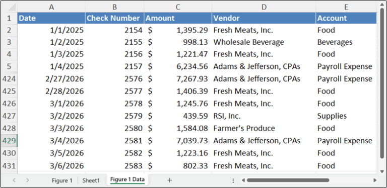
Once you familiarize yourself with the arguments – especially the required ones – creating a formula-driven PivotTable is easy. For example, consider the date pictured below in Figure 1 (with multiple rows hidden for presentation purposes).

To generate a PIVOTBY-driven report using the data available in Figure 1, enter the following formula into Excel: =PIVOTBY(A2:A431,D2:D431,C2:C431,SUM)
Upon entering the formula and pressing ENTER, PIVOTBY generates a report similar to that pictured in Figure 2 (with multiple columns and rows hidden for presentation purposes).

Now, to the power of using the feature. The optional arguments available with the function give you much more control over how your formula-driven PivotTables summarize and present their data. For instance, modifying the formula to indicate you want to generate an average instead of a sum is easily done by changing the formula, as shown in the following formula: =PIVOTBY(A2:A431,D2:D431,C2:C431,AVERAGE)
Advantages Associated With PIVOTBY
PIVOTBY provides accounting and financial professionals with numerous options and advantages when generating PivotTable-like reports. For example, the function allows users to generate summaries of data within cells. This trait means that creating a separate reporting object in the form of a PivotTable is unnecessary. As a result, PIVOTBY could be advantageous when creating Excel-based dashboards.
Another advantage associated with PIVOTBY is the dynamic nature of the function. Because PIVOTBY is an Excel function, it updates its calculations every time the workbook changes. Thus, users no longer need to refresh a PivotTable to ensure that they are looking at up-to-date summarizations.
Additionally, PIVOTBY offers a virtually unlimited number of calculations. For example, you can use PIVOTBY to create a summary of transactions by vendor, an average of sales revenue by customer, and a count of purchase orders by supplier. You are no longer bound by some of the limitations associated with traditional PivotTables.
Accounting And Financial Potential Uses Of PIVOTBY
For accounting and financial professionals, the potential uses of PIVOTBY are virtually limitless For example, you can use PIVOTBY to generate real-time, up-to-date budget versus actual comparisons. To illustrate, suppose the data in Column A of a report contains the department name, Column B contains month labels, and Column C contains expense values. In this case, you could create the following PIVOTBY report based on the following function: =PIVOTBY(A2:D100, A2:A100, B2:B100, C2:C100, SUM)
Other examples of reports that you might consider re-configuring include sales analysis reports, vendor performance reports, and employee timesheet summaries.
Summary
Excel’s PIVOTBY function provides a welcome addition to the application’s function library. With PIVOTBY, you can generate reports and data summaries that are more flexible and potentially more powerful than PivotTable-based reports. Although generating a PIVOTBY-based report differs from that of generating a PivotTable, most users will adapt quickly with just a bit of practice. Therefore, if you’re looking to create a report that capitalizes on the advantages of PivotTables, but offers more flexibility and functionality, check out Excel’s new function.
You can learn more about PIVOTBY at https://k2e.fyi/pivotby.
At K2 Enterprises, our commitment lies in providing unwavering support and expert instruction to CPAs. Explore the wealth of resources on our website, where you’ll find valuable insights on selecting the most suitable accounting software, ensuring your firm is equipped with the right tools for the journey ahead. If you work in accounting or finance, K2 Enterprises provides continuing education programs to enhance your skills and credentials. Need help learning how to solve your business’s accounting technology needs and selecting the right software for accounting or CPA Firms? Visit us at k2e.com, where we make sophisticated technology understandable to anyone through our conferences, seminars, or on-demand courses.


